1 R Programming Language

1.1 Use R as a calculator

To start learning R, just start entering equations directly at the command prompt > and press enter. So, 3+4 will give you result 7. Common mathematical operators are listed in table 1.1.

Table 1.1: Common Mathematical Operators in R

Operator/ function	Meaning	Example
+	Addition	4 + 5 is 9
-	Substraction	4 - 5 is -1
*	Multiplication	4 * 5 is 20
/	Division	4/5 is 0.8
^	Exponent	2^4 is 16
%%	Modulus (Remainder from division)	15 %% 12 is 3
%/%	Integer Division	15 %/% 12 is 1

Strings or Characters have to be enclosed in single ' or double" quotes (more on strings in section 1.3.4). So a few examples of calculations that can be performed in R could be-

4 + 3 ^ 2

## [1] 13

8 * (9 + 4)

## [1] 104

Note that R follows common mathematical order of precedence while evalauting expressions. That may be changed using simple parenthesis i.e. (). Also note that other brackets/braces i.e. curly braces {} and [] have been assigned different meaning, so to change nested order of operations only () may be used.

1.2 Object Assignment

R is an object-oriented language.³ This means that objects are created and stored in R environment so that they can be used later.

So what is an object? An object can be something as simple as a number (value) that can be assigned to a variable. Think of it like this; Suppose we have greet each user by his/her name prefixing hello to his/her name. Now user’s name may be saved in our work environment for later use. Thus, once the user name is saved in a variable then can be retrieved later on, by calling the variable name instead of asking the user name again and again. An object can be also be a data-set or complex model output or some function. Thus, an object created in R can hold multiple values.

The other important thing about objects is that objects are created in R, using the assignment operator <-. Use of equals sign = to set something as an object is not recommended thought it will work properly in some cases. For now we will stick with the assignment operator, and interpret it as the left side is the object name that is storing the object information specified on the right side. If -> right hand side assignment is used, needless to say things mentioned above will interchange.

# user name
user_name <- 'Anil Goyal'

# when the above variable is called
user_name

## [1] "Anil Goyal"

Case sensitive nature: Names of variables even all objects in R are case sensitive, and thus user, USER and useR; all are different variables.

1.3 Atomic data types in R

We have seen that objects in R can be created to store some values/data. Even these objects can contain other objects as well. So a question arises, what is the most atomic/basic data type in R. By atomic we mean that the object cannot be split any further. Thus, the atomic objects created in R can be thought of variables holding one single value. E.g. user’s name, user’s age, etc. Now atomic objects created in R can be of six types-

• logical (or Boolean i.e. TRUE FALSE etc.)
• integer (having non-decimal numeric values like 0, 1, etc.)
• double ( or floating decimal type i.e. having numeric values in decimal i.e. 1.0 or 5.25, etc.)
• character (or string data type having some alphanumeric value)
• complex (numbers having both real and imaginary parts e.g. 1+1i)
• raw (not discussed here)

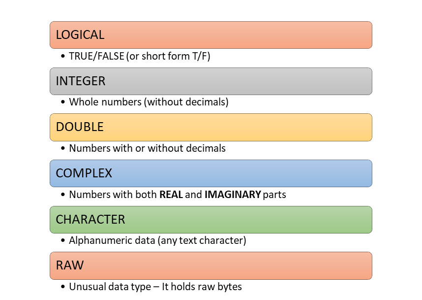
Figure 1.1: Data types in R

Let us discuss all of these.

Note: We will use a pre-built function typeof() to check the type of given value/variable. However, functions as such will be discussed later-on.

1.3.1 Logical

In R logical values are stored as either TRUE or FALSE (all in caps)

TRUE

## [1] TRUE

typeof(TRUE)

## [1] "logical"

my_val <- TRUE
typeof(my_val)

## [1] "logical"

NA: There is one special type of logical value i.e. NA (short for Not Available). This is used for missing data.

Remember missing data is not an empty string. The difference between the two is explained in section 1.3.4.

1.3.2 Integer

Numeric values can either be integer (i.e. without a floating point decimal) or with a floating decimal value (called double in r). Now integers in R are differentiated by a suffix L. E.g.

my_val1 <- 2L
typeof(my_val1)

## [1] "integer"

typeof(2)

## [1] "double"

1.3.3 Double

Numeric values with decimals are stored in objects of type double. It should be kept in mind that if storing an integer value directly to a variable, suffix L must be used otherwise the object will be stored as double type as shown in above example.

In double type, exponential formats or hexadecimal formats to store these numerals may also be used.

my_val2 <- 2.5
my_val3 <- 1.23e4
my_val4 <- 0xcafe # hexadecimal format (prefixed by 0x)

typeof(my_val2)

## [1] "double"

typeof(my_val3)

## [1] "double"

typeof(my_val4)

## [1] "double"

Note: Suffix L may also be used with numerals in hexadecimal (e.g. 0xcafeL) or exponential formats (e.g. 1.23e4L), which will coerce these numerals in integer format.

typeof(0xcafeL)

## [1] "integer"

Thus, both integer and double data types may be understood in R as having sub-types of numeric data. There are three other types of special numerals (specifically doubles) Inf, -Inf and NaN. The first two are infinity (positive and negative) and the last one denotes an indefinite number (NaN short for Not a Number).

1/0

## [1] Inf

-45/0

## [1] -Inf

0/0

## [1] NaN

1.3.4 Character

Strings are stored in R as a character type. Strings should either be surrounded by single quotes '' or double quotes ""⁴.

my_val5 <- 'Anil Goyal'
my_val6 <- "Anil Goyal"
my_val7 <- "" # empty string
my_missing_val <- NA # missing value

typeof(my_val5)

## [1] "character"

typeof(my_val6)

## [1] "character"

typeof(my_val7)

## [1] "character"

typeof(my_missing_val)

## [1] "logical"

[Notes:\\](Notes:){.uri} 1. Though NA is basically of type logical yet it will be used to store missing values in any other data type also as shown in subsequent chapter(s). 2. Special characters are escaped with \; Type ?Quotes in console and check documentation for full details. 3. A simple use of \ escape character may be to use " or ' within these quotes. Check Example-3 below.

Example-1: Usage of double and single quote interchangeably.

my_val8 <- "R's book"
my_val8

## [1] "R's book"

Example-2: Usage of escape character.

cat("This is first line.\nThis is new line")

## This is first line.
## This is new line

Example-3: Usage of escape character to store single/double quotes as string themselves.

cat("\' is single quote and \" is double quote")

## ' is single quote and " is double quote

Note: If absence of indices has been noticed in above code output, learn more about cat function here.

1.3.5 NULL

NULL (note: all caps) is a specific data type used to create an empty vector. Even this NULL can be used as a vector in itself.

typeof(NULL)

## [1] "NULL"

vec <- 1:5
vec

## [1] 1 2 3 4 5

vec <- NULL
vec

## NULL

1.3.6 Complex

Complex numbers are made up of real and imaginary parts. As these will not be used in the data analysis tasks, it is not discussed in detail here.

my_complex_no <- 1+1i
typeof(my_complex_no)

## [1] "complex"

1.4 Data structures/Object Types in R

Objects in R can be either homogeneous or heterogeneous.

Figure 1.2: Objects/Data structures in R, can either be homogeneous (left) or heterogeneous (right)

Homogeneous objects

1.4.1 Vectors

What is a vector? A vector is simply a collection of values/data of same type.

Figure 1.3: Vectors are homegeneous data structures in R

1.4.1.1 Simple vectors (Unnamed vectors)

Though, Vector is the most atomic data type used in R, yet it can hold multiple values (of same type) simultaneously. In fact vector is a collection of multiple values of same type. So why vector is atomic when it can hold multiple values? You may have noticed a [1] printed at the start of line of output whenever a variable was called/printed. This [1] actually is the index of that element. Thus, in R instead of having scalar(s) as most atomic type, we have vector(s) containing only one element. Whenever a vector is called all the values stored in it are displayed with its index at the start of each new line only.

Even processing of multiple values simultaneously, stored in a vector, to produce a desired output, is one of the most powerful strengths of R. The three variables shown in the figure below, all are vectors.

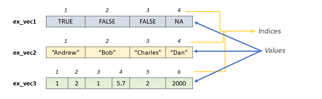
Figure 1.4: Examples of Vectors

How to create a vector? Vectors in R are created using either -

• c() function which is shortest and most commonly used function in r. The elements are concatenated (and hence the shortcut c for this function) using a comma , ; OR
• vector() produces vector of given length and mode.

my_vector <- c(1, 2, 3)
my_vector

## [1] 1 2 3

my_vector2 <- vector(mode = 'integer', length = 15)
my_vector2

##  [1] 0 0 0 0 0 0 0 0 0 0 0 0 0 0 0

Function c() can also be used to join two or more vectors.

vec1 <- c(1, 2)
vec2 <- c(11, 12)
vec3 <- c(vec1, vec2)
vec3

## [1]  1  2 11 12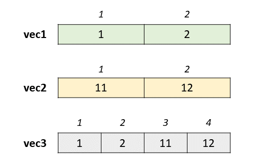

Figure 1.5: Vector Concatenation

Useful Functions to create new vectors

There are some more useful functions to create new vectors in R, which we should discuss here as we will be using these vectors in subsequent chapters.

Generate integer sequences with Colon Operator :

This function generates a sequence from the number preceding : to next specified number, in arithmetical difference of 1 or -1 as the case may be. Notice that output vector type is of integer.

1:25

##  [1]  1  2  3  4  5  6  7  8  9 10 11 12 13 14 15 16 17 18 19 20 21 22 23 24 25

25:30

## [1] 25 26 27 28 29 30

10:1

##  [1] 10  9  8  7  6  5  4  3  2  1

typeof(2:250)

## [1] "integer"

Note: One of the common mistakes with colon operator is assuming its operator precedence. In R, colon operator has calculation precedence over any mathematical operator. Think of outputs you may get with these-

n <- 5
1:n+1
1:n*2

Generate specific sequences with function seq

This function generates a sequence from a given number to another number, similar to :, but it gives us more control over the output desired. We can provide the difference specifically (double type also) in the by argument. Otherwise if length.out argument is provided it calculates the difference automatically.

seq(1, 5, by = 0.3)

##  [1] 1.0 1.3 1.6 1.9 2.2 2.5 2.8 3.1 3.4 3.7 4.0 4.3 4.6 4.9

seq(1, 2, length.out = 11)

##  [1] 1.0 1.1 1.2 1.3 1.4 1.5 1.6 1.7 1.8 1.9 2.0

Repeat a pattern/vector with function rep

As the name suggests rep is short for repeat and thus it repeat a given element, a given number of times.

rep('repeat this', 5)

## [1] "repeat this" "repeat this" "repeat this" "repeat this" "repeat this"

# We can even repeat already created vectors
vec <- c(1, 10)
rep(vec, 5)

##  [1]  1 10  1 10  1 10  1 10  1 10

rep(vec, each = 5) # notice the difference in results

##  [1]  1  1  1  1  1 10 10 10 10 10

Generate english alphabet with LETTERS / letters

These are two inbuilt vectors in R having all 26 alphabets in upper and lower cases respectively.

LETTERS

##  [1] "A" "B" "C" "D" "E" "F" "G" "H" "I" "J" "K" "L" "M" "N" "O" "P" "Q" "R" "S"
## [20] "T" "U" "V" "W" "X" "Y" "Z"

letters

##  [1] "a" "b" "c" "d" "e" "f" "g" "h" "i" "j" "k" "l" "m" "n" "o" "p" "q" "r" "s"
## [20] "t" "u" "v" "w" "x" "y" "z"

Generate gregorian calendar month names with month.name / month.abb

month.name

##  [1] "January"   "February"  "March"     "April"     "May"       "June"     
##  [7] "July"      "August"    "September" "October"   "November"  "December"

month.abb

##  [1] "Jan" "Feb" "Mar" "Apr" "May" "Jun" "Jul" "Aug" "Sep" "Oct" "Nov" "Dec"

1.4.1.2 Named Vectors

Vectors in R, can be named also, i.e. where each of the element has a name. E.g.

ages <- c(A = 10, B = 20, C = 15)
ages

##  A  B  C 
## 10 20 15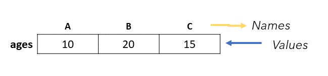

Figure 1.6: Vector elements can have names

Note here that while assigning names to each element, the names are not enclosed in quotes similar to variable assignment. Also notice that this time R has not printed the numeric indices/index of first element (on each new line). There are other ways to assign names to an existing vector. We can use names() function, which displays the names of all elements in that vector ( and this time in quotes as these are displayed in a vector).

names(ages)

## [1] "A" "B" "C"

Using this function we can assign names to existing vector. See

vec1

## [1] 1 2

names(vec1) <- c('first_element', 'second_element')
vec1

##  first_element second_element 
##              1              2

Names may also be assigned using setNames() while creating the vector simultaneously.

new_vec <- setNames(1:26, LETTERS)
new_vec

##  A  B  C  D  E  F  G  H  I  J  K  L  M  N  O  P  Q  R  S  T  U  V  W  X  Y  Z 
##  1  2  3  4  5  6  7  8  9 10 11 12 13 14 15 16 17 18 19 20 21 22 23 24 25 26

Function unname() may be used to remove all names. Even all the names can be removed by assigning NULL to names of that vector. Also remember that unname does not modify vector in place. To have this change we will have to assigned unnamed vector to that vector again. Check this,

unname(new_vec)

##  [1]  1  2  3  4  5  6  7  8  9 10 11 12 13 14 15 16 17 18 19 20 21 22 23 24 25
## [26] 26

new_vec

##  A  B  C  D  E  F  G  H  I  J  K  L  M  N  O  P  Q  R  S  T  U  V  W  X  Y  Z 
##  1  2  3  4  5  6  7  8  9 10 11 12 13 14 15 16 17 18 19 20 21 22 23 24 25 26

new_vec <- unname(new_vec)
new_vec

##  [1]  1  2  3  4  5  6  7  8  9 10 11 12 13 14 15 16 17 18 19 20 21 22 23 24 25
## [26] 26

Type coercion

There are occasions when different classes of R objects get mixed together. Sometimes this happens by accident but it can also happen on purpose. Let us deal with each of these.

But prior to this let us learn how to check the type of a vector. Of course we can check the type of any vector using function typeof() but what if we want to check whether any vector is of a specific type. So there are is.*() functions to check this, and all these functions return either TRUE or FALSE.

• is.logical()
• is.integer()
• is.double()
• is.character()
• is.complex()

is.integer(1:10)

## [1] TRUE

is.logical(LETTERS)

## [1] FALSE

Implicit Coercion

As already stated, vector is the most atomic data object in R. Even all the elements of a vector (having multiple elements) are vectors in themselves. We have also discussed that vectors are homogeneous in types. So what happens when we try to mix elements of different types in a vector.

In fact when we try to mix elements of different types in a vector, the resultant vector is coerced to the type which is most feasible. Since a numeral say 56 can easily be converted into a complex number (56+0i) or character ("56"), but alphabet say A, cannot be converted into a numeral, the atomic data types normally follow the order of precedence, tabulated in table 1.2.

Table 1.2: Order of Precedence for Atomic Data Types

Rank	Type
1	Character
2	Complex
3	Double
4	Integer
5	Logical

For e.g. in the following diagram, notice all individual elements in first vector. Out of the types of all elements therein, character type is having highest rank and thus resultant vector will be silently coerced to a character vector. Similarly, second and third vectors are coerced to double (second element) and integer (first element) respectively.

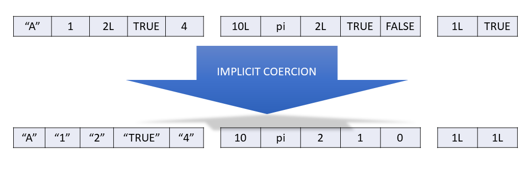
Figure 1.7: Implicit Coercion of Vectors

It is also important to note here that this implicit coercion is without any warning and is silently performed. This implicit coercion is also carried out when two (or more) vectors having different data types are concatenated together.

Example- vec is an existing vector of type integer. When we try to add an extra element say of character type, vec type is coerced to character.

vec <- 1:5
typeof(vec)

## [1] "integer"

vec <- append(vec, 'ABCD')
typeof(vec)

## [1] "character"

R also implicitly coerces vectors to appropriate type when we try to perform calculations on vectors of other types. Example

(TRUE == FALSE) + 1

## [1] 1

typeof(TRUE + 1:100)

## [1] "integer"

typeof(FALSE + 56)

## [1] "double"

Explicit Coercion

We can explicitly coerce by using an as.*() function, like as.logical(), as.integer(), as.double(), or as.character(). Failed coercion of strings generates a warning and a missing value:

as.double(c(TRUE, FALSE))

## [1] 1 0

as.integer(c(1, 'one', 1L))

## Warning: NAs introduced by coercion

## [1]  1 NA  1

1.4.1.3 Coercion precedence

Sometimes, inside R both coercion happen at same time. So which one to precede other? Actually, implicit coercion will precede explicit coercion always. Consider this example. However, without seeing the result try to guess the output.

as.logical(c('TRUE', 1))

## [1] TRUE   NA

Explanation: the vector c('TRUE', 1) coerces to c('TRUE', '1') due to implicit coercion first and thereafter explicit coercion forces second element as.logical('1') to NA. Though as.logical(1) would have resulted into TRUE but as.logical("1") would result into NA.

Checking dimensions

Now a vector can have n number of vectors (recall that each element is a vector in itself) and at times we may need to check how many elements a given vector contains. Using function length(), we can check the number of elements.

length(1:100)

## [1] 100

length(LETTERS)

## [1] 26

length('LENGTH') # If you thought its output should have been 6, check again.

## [1] 1

1.4.2 Matrix (Matrices)

Matrix (or plural matrices) is a two dimensional arrangement (similar to a matrix in linear algebra and hence its name) of elements of again same type as in vectors. E.g.

\[\begin{array}{ccc} x_{11} & x_{12} & x_{13}\\ x_{21} & x_{22} & x_{23} \end{array}\]

Thus, matrices are vectors with an attribute named dimension.

The dimension attribute is itself an integer vector of length 2 (number of rows, number of columns).

Create a new matrix

A new matrix can be created using function matrix() where a vector is given which is to be converted into a matrix and either number of rows nrow or number of columns ncol may be given.

matrix(1:12, nrow = 3)

##      [,1] [,2] [,3] [,4]
## [1,]    1    4    7   10
## [2,]    2    5    8   11
## [3,]    3    6    9   12

matrix(1:12, ncol=3)

##      [,1] [,2] [,3]
## [1,]    1    5    9
## [2,]    2    6   10
## [3,]    3    7   11
## [4,]    4    8   12

Another useful argument is byrow which by default is FALSE. So if it is explicitly changed, we get

matrix(1:12, ncol=3, byrow = TRUE)

##      [,1] [,2] [,3]
## [1,]    1    2    3
## [2,]    4    5    6
## [3,]    7    8    9
## [4,]   10   11   12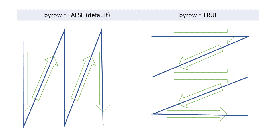

Figure 1.8: Arrangement of Matrix, if byrow argument is used

Matrix can be of any type. But rules of explicit and implicit coercion (as explained in vectors) also apply here.

matrix(LETTERS, nrow = 2)

##      [,1] [,2] [,3] [,4] [,5] [,6] [,7] [,8] [,9] [,10] [,11] [,12] [,13]
## [1,] "A"  "C"  "E"  "G"  "I"  "K"  "M"  "O"  "Q"  "S"   "U"   "W"   "Y"  
## [2,] "B"  "D"  "F"  "H"  "J"  "L"  "N"  "P"  "R"  "T"   "V"   "X"   "Z"

matrix(c(LETTERS, 1:4), nrow=5)

##      [,1] [,2] [,3] [,4] [,5] [,6]
## [1,] "A"  "F"  "K"  "P"  "U"  "Z" 
## [2,] "B"  "G"  "L"  "Q"  "V"  "1" 
## [3,] "C"  "H"  "M"  "R"  "W"  "2" 
## [4,] "D"  "I"  "N"  "S"  "X"  "3" 
## [5,] "E"  "J"  "O"  "T"  "Y"  "4"

Names in matrices

Similar to vectors, rows or columns or both in matrices may have names. Check ?matrix() for complete documentation.

Dimension

To check dimension of a matrix we can use dim() (short for dimension) (similar to length in case of vectors) which will return a vector with two numbers (rows first, followed by columns).

my_mat <- matrix(c(LETTERS, 1:4), nrow=5)
dim(my_mat)

## [1] 5 6

This gives us another method to create matrix from a vector. See

my_mat2 <- 1:10
dim(my_mat2) <- c(2,5)
my_mat2

##      [,1] [,2] [,3] [,4] [,5]
## [1,]    1    3    5    7    9
## [2,]    2    4    6    8   10

Have a check on replication

What happens when product of given dimensions is less than or greater than given vector to be converted. It replicates but it is advised to check these properly as resultant vector may not be as desired. Check these cases, and notice when R gives result silently and when with a warning.

matrix(1:10, nrow=5, ncol=5)

## Warning in matrix(1:10, nrow = 5, ncol = 5): data length differs from size of
## matrix: [10 != 5 x 5]

##      [,1] [,2] [,3] [,4] [,5]
## [1,]    1    6    1    6    1
## [2,]    2    7    2    7    2
## [3,]    3    8    3    8    3
## [4,]    4    9    4    9    4
## [5,]    5   10    5   10    5

matrix(1:1000, nrow=2, ncol=3)

## Warning in matrix(1:1000, nrow = 2, ncol = 3): data length [1000] is not a
## sub-multiple or multiple of the number of columns [3]

##      [,1] [,2] [,3]
## [1,]    1    3    5
## [2,]    2    4    6

Combining matrices

Using cbind() or rbind() we can combine two matrices column-wise or row-wise respectively.

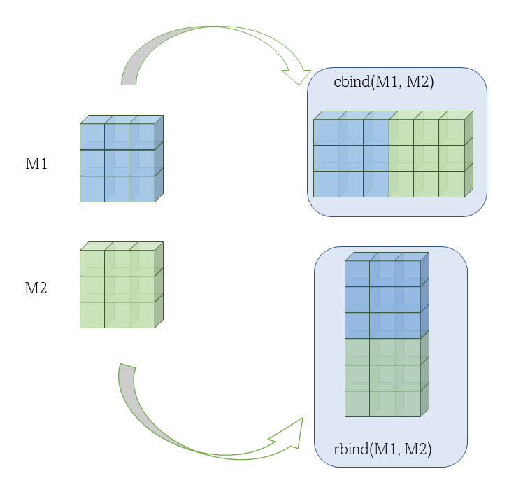
Figure 1.9: Binding of Two or more matrices together

See these two examples.

mat1 <- matrix(1:4, nrow = 2)
mat2 <- matrix(5:8, nrow = 2)
cbind(mat1, mat2)

##      [,1] [,2] [,3] [,4]
## [1,]    1    3    5    7
## [2,]    2    4    6    8

Example-2

rbind(mat1, mat2)

##      [,1] [,2]
## [1,]    1    3
## [2,]    2    4
## [3,]    5    7
## [4,]    6    8

1.4.3 Arrays

Till now we have seen that elements in one dimension are represented as vectors and in two dimension as matrices. So a question arises here, how many dimensions we can have. Actually we can have n number of dimensions in r, in object type array, but they’ll become increasingly difficult to comprehend and are not thus discussed here. Check these however for your understanding,

array(1:24, dim = c(3,2,4)) # a three dimensional array

## , , 1
## 
##      [,1] [,2]
## [1,]    1    4
## [2,]    2    5
## [3,]    3    6
## 
## , , 2
## 
##      [,1] [,2]
## [1,]    7   10
## [2,]    8   11
## [3,]    9   12
## 
## , , 3
## 
##      [,1] [,2]
## [1,]   13   16
## [2,]   14   17
## [3,]   15   18
## 
## , , 4
## 
##      [,1] [,2]
## [1,]   19   22
## [2,]   20   23
## [3,]   21   24

Try creating 4 or 5 dimensional arrays in your console and see the results.

Further properties of vectors, matrices will be discussed in next chapter on sub-setting and indexing where we will learn how to retrieve specific elements of vector/matrices/etc. But till now we have created objects which have elements of same type. What if we want to have different types of elements/data retaining their types, together in a single variable? Answer is in next section, where we will discuss hetergeneous objects.

Heterogeneous objects

1.4.4 Lists

So lists are used when we want to combine elements of different types together. Function used to create a list is list(). Check this

list(1, 2, 3, 'My string', TRUE)

## [[1]]
## [1] 1
## 
## [[2]]
## [1] 2
## 
## [[3]]
## [1] 3
## 
## [[4]]
## [1] "My string"
## 
## [[5]]
## [1] TRUE

Pictorially this list can be depicted as

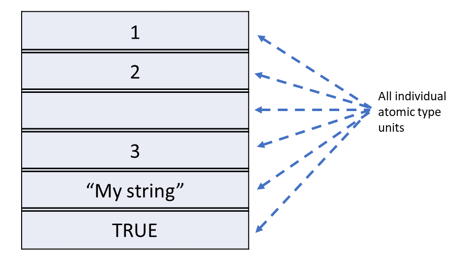
Figure 1.10: A list in R is a heterogeneous object

Interestingly list can contain vectors, matrices, arrays as individual elements. See

list(1:3, LETTERS, TRUE, my_mat2)

## [[1]]
## [1] 1 2 3
## 
## [[2]]
##  [1] "A" "B" "C" "D" "E" "F" "G" "H" "I" "J" "K" "L" "M" "N" "O" "P" "Q" "R" "S"
## [20] "T" "U" "V" "W" "X" "Y" "Z"
## 
## [[3]]
## [1] TRUE
## 
## [[4]]
##      [,1] [,2] [,3] [,4] [,5]
## [1,]    1    3    5    7    9
## [2,]    2    4    6    8   10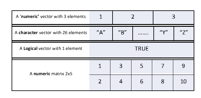

Figure 1.11: A list in R, can contain vector, matrices, array or even lists

Similar to vectors these elements can be named also.

list(first_item = 1:5, second_item = my_mat2)

## $first_item
## [1] 1 2 3 4 5
## 
## $second_item
##      [,1] [,2] [,3] [,4] [,5]
## [1,]    1    3    5    7    9
## [2,]    2    4    6    8   10

OR

my_list <- list(first=c(A=1, B=2, C=3),second=my_mat2)
my_list

## $first
## A B C 
## 1 2 3 
## 
## $second
##      [,1] [,2] [,3] [,4] [,5]
## [1,]    1    3    5    7    9
## [2,]    2    4    6    8   10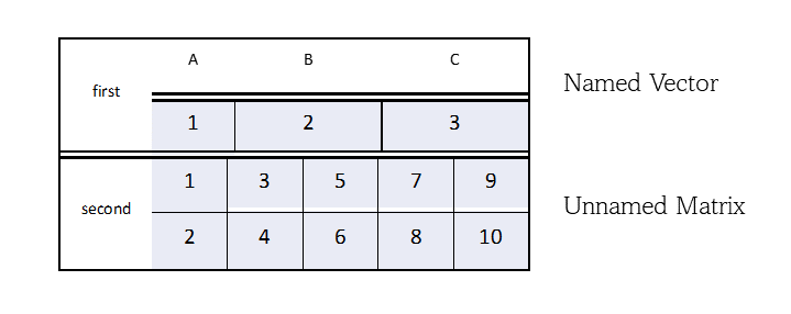

Figure 1.12: Similar to vector elements, the elements in list can be named also

OR

More interestingly, lists can even contain another lists.

my_list2 <- list(my_list, new_item = LETTERS)
my_list2

## [[1]]
## [[1]]$first
## A B C 
## 1 2 3 
## 
## [[1]]$second
##      [,1] [,2] [,3] [,4] [,5]
## [1,]    1    3    5    7    9
## [2,]    2    4    6    8   10
## 
## 
## $new_item
##  [1] "A" "B" "C" "D" "E" "F" "G" "H" "I" "J" "K" "L" "M" "N" "O" "P" "Q" "R" "S"
## [20] "T" "U" "V" "W" "X" "Y" "Z"

Number of items at first level can be checked using length as in vectors. Checking number of items in second level onward will be covered in subsequent chapter(s).

length(my_list)

## [1] 2

length(my_list2) # If you thought its output should have been 3, think again.

## [1] 2

1.4.5 Data Frame

Data frames are used to store tabular data (or rectangular) in R. They are an important type of object in R.

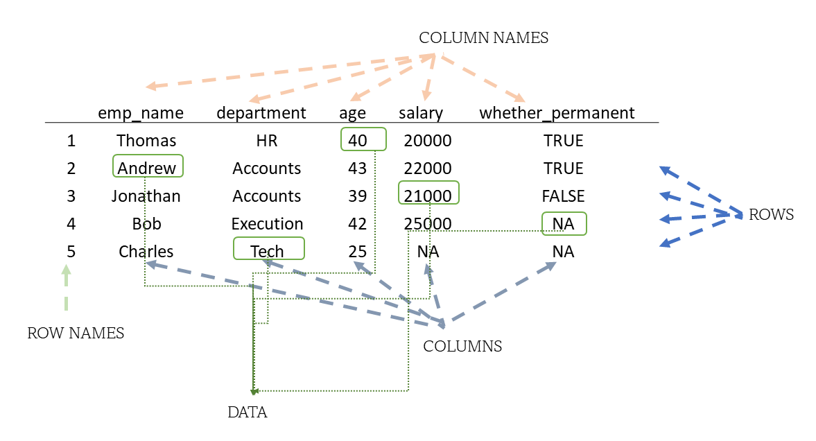
Figure 1.13: An example data frame

Data frames are represented as a special type of list where every element of the list has to have the same length. Each element of the list can be thought of as a column and the length of each element of the list is the number of rows.

Figure 1.14: A data frame in R, is just a special kind of list

Unlike matrices, data frames can store different classes of objects in each column. (Remember that matrices must have every element be the same class).

To create a data frame from scratch we will use function data.frame(). See

my_df <- data.frame(emp_name = c('Thomas', 'Andrew', 'Jonathan', 'Bob', 'Charles'),
                    department = c('HR', 'Accounts', 'Accounts', 'Execution', 'Tech'),
                    age = c(40, 43, 39, 42, 25),
                    salary = c(20000, 22000, 21000, 25000, NA),
                    whether_permanent = c(TRUE, TRUE, FALSE, NA, NA))
my_df

##   emp_name department age salary whether_permanent
## 1   Thomas         HR  40  20000              TRUE
## 2   Andrew   Accounts  43  22000              TRUE
## 3 Jonathan   Accounts  39  21000             FALSE
## 4      Bob  Execution  42  25000                NA
## 5  Charles       Tech  25     NA                NA

Note that R, on its own, has allocated row names that are numbers to each of the row on its own.

Of course at most of the times we will have data frames ready for us to analyse and thus we will learn to import/read external data in r, in subsequent chapters. To check dimensions of a data frame use dim as in matrix.

dim(my_df)

## [1] 5 5

Thus, the object types in R, can be depicted as in adjoining figure.

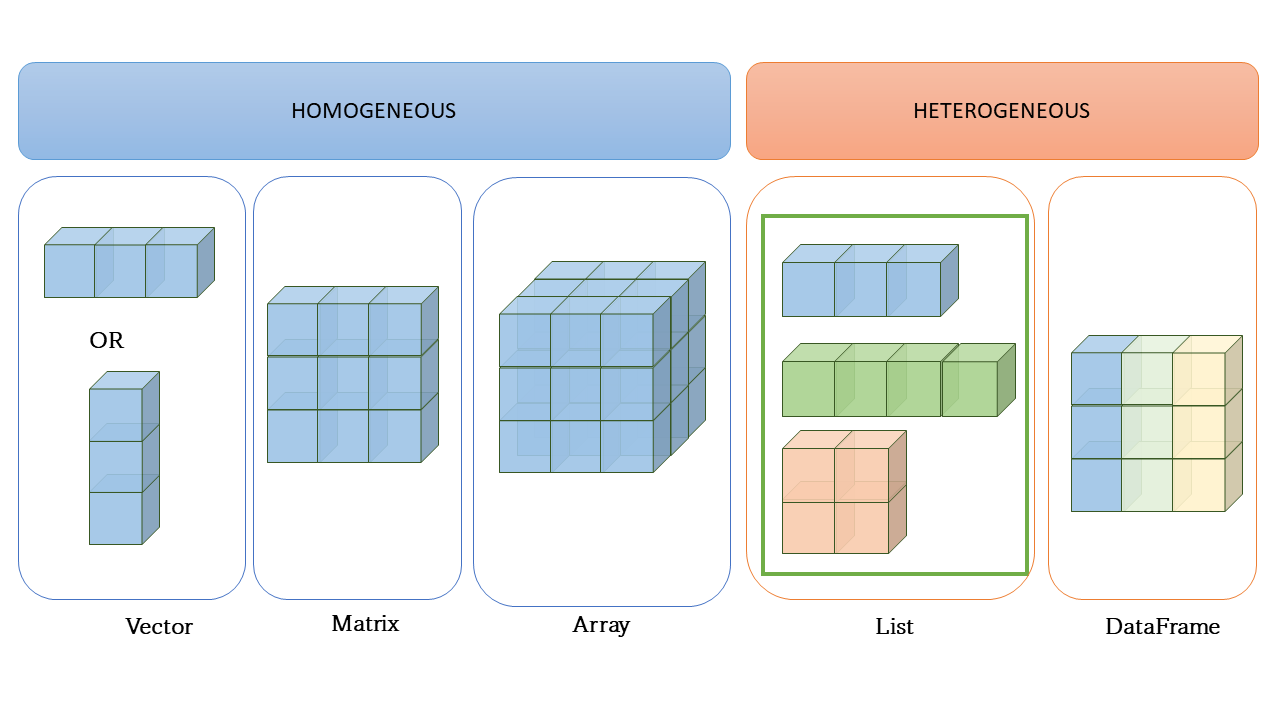
Figure 1.15: Most important Data structures, in R

1.5 Other Data types

Of course, there are other data types in R of which three are particularly useful factor, date and date-time. These types are actually built over the base atomic types, integer, double and double respectively and that’s why these are being discussed separately. These types are built as S3 objects in R, and users may also define their own data types in object oriented programming. OOP being concept of core programming concepts and therefore are out of the scope here.

However, to understand the S3 objects better, we have to understand that atomic objects (for the sake of simplicity consider only vectors) can have attributes.

Example One of the attributes that each vector has is names, which for unnamed vector is empty (NULL). Attributes of any object can be viewed/called from function attributes().

# Let us create a vector
vec <- 1:26
# Convert this to a named vector using function setNames()
# This function takes first argument as vector
# Second argument should be a character vector of equal length.
vec <- setNames(vec, LETTERS)
# let's check what are the attributes of `vec`
attributes(vec)

## $names
##  [1] "A" "B" "C" "D" "E" "F" "G" "H" "I" "J" "K" "L" "M" "N" "O" "P" "Q" "R" "S"
## [20] "T" "U" "V" "W" "X" "Y" "Z"

Using attr() we may assign any new attribute to any R object/variable.

# Let's also assign a new attribute say `x` having value "New Attribute" to `vec`
attr(vec, "x") <- "New Attribute"
# Now let's check its attributes again
attributes(vec)

## $names
##  [1] "A" "B" "C" "D" "E" "F" "G" "H" "I" "J" "K" "L" "M" "N" "O" "P" "Q" "R" "S"
## [20] "T" "U" "V" "W" "X" "Y" "Z"
## 
## $x
## [1] "New Attribute"

We can see, in above example, how a new attribute has been added to a vector. It should have been clear by now that apart from names, other attributes may also be assigned to a vector.

1.5.1 Factors

A factor is a vector that can contain only predefined values. It is used to store categorical data. Factors are built on top of an integer vector with two attributes: a class, ‘factor’, which makes it behave differently from regular integer vectors, and levels, which defines the set of allowed values. To create factors we will use function factor.

fac <- factor(c('a', 'b', 'c', 'a'))
fac

## [1] a b c a
## Levels: a b c

typeof(fac) # notice its output

## [1] "integer"

attributes(fac)

## $levels
## [1] "a" "b" "c"
## 
## $class
## [1] "factor"

So if typeof of a factor is returning integer, how will we check its type? We may use class or is.factor in this case.

class(fac)

## [1] "factor"

is.factor(fac)

## [1] TRUE

Now a factor can be ordered also. We may use its argument ordered = TRUE along with another argument levels.

my_degrees <- c("PG", "PG", "Doctorate", "UG", "PG")
my_factor <- factor(my_degrees, levels = c('UG', 'PG', 'Doctorate'), ordered = TRUE)
my_factor # notice output here

## [1] PG        PG        Doctorate UG        PG       
## Levels: UG < PG < Doctorate

is.ordered(my_factor)

## [1] TRUE

Another argument labels can also be used to display the labels, which may be different from levels.

my_factor <- factor(my_degrees, levels = c('UG', 'PG', 'Doctorate'), 
                    labels = c("Under-Graduate", "Post Graduate", "Ph.D"),
                    ordered = TRUE)
my_factor # notice output here

## [1] Post Graduate  Post Graduate  Ph.D           Under-Graduate Post Graduate 
## Levels: Under-Graduate < Post Graduate < Ph.D

is.factor(c(my_factor, "UG"))

## [1] FALSE

Attribute levels can be used as a function to retrieve/modify these.

levels(my_factor)

## [1] "Under-Graduate" "Post Graduate"  "Ph.D"

levels(my_factor) <- c("Grad", "Masters", "Doctorate")
my_factor

## [1] Masters   Masters   Doctorate Grad      Masters  
## Levels: Grad < Masters < Doctorate

Remember that while factors look like (and often behave like) character vectors, they are built on top of integers. Try to think of output of this is.factor(c(my_factor, "UG")) before running it in your console.

We will learn about these data types in detail in chapter 31.

1.5.2 Date

Date vectors are built on top of double vectors. They have class “Date” and no other attributes. A common way to create date vectors in R, is converting a character string to date using as.Date() (see case carefully),

my_date <- as.Date("1970-01-31")
my_date

## [1] "1970-01-31"

attributes(my_date)

## $class
## [1] "Date"

Do check other arguments of as.Date by running ?as.Date() in your console. To check whether a given variable is of type Date in r, there is no function like is.Date in base r, so we may use inherits() in this case.

inherits(my_date, 'Date')

## [1] TRUE

1.5.3 Date-time (POSIXct)

Times are represented by the POSIXct or the POSIXlt class.

• POSIXct is just a very large integer under the hood. It use a useful class when you want to store times in something like a data frame.
• POSIXlt is a list underneath and it stores a bunch of other useful information like the day of the week, day of the year, month, day of the month.

my_time <- Sys.time()
my_time

## [1] "2024-12-13 15:32:56 IST"

class(my_time)

## [1] "POSIXct" "POSIXt"

my_time2 <- as.POSIXlt(my_time)
class(my_time2)

## [1] "POSIXlt" "POSIXt"

names(unclass(my_time2))

##  [1] "sec"    "min"    "hour"   "mday"   "mon"    "year"   "wday"   "yday"  
##  [9] "isdst"  "zone"   "gmtoff"

1.5.4 Duration (difftime)

Duration, which represent the amount of time between pairs of dates or date-times, are stored in difftimes. Difftimes are built on top of doubles, and have a units attribute that determines how the integer should be interpreted.

two_days <- as.difftime(2, units = 'days')
two_days

## Time difference of 2 days

These over the top, data types will be discussed in more detail in chapter 24.