34 Visualising Text analytics through Wordcloud, etc.

The content is under development is following is not finalised.

34.1 Frequency plots

34.2 Wordclouds

34.2.1 Step-1:Prepare data and load libraries

As an example we will create a word cloud with Budget Speech made by Finance Minister during her Budget speech³⁶ 2022-23. All of the budget speech is available in file called budget.txt.

Load Libraries

library(tidyverse)
library(tidytext) #install.packages("tidytext")
library(wordcloud) #install.packages("wordcloud")
library(ggtext)
library(ggalt)
library(ggthemes)
library(ggpubr)
library(conflicted)
conflicts_prefer(dplyr::filter)

Load data

dat <- read.table('data/budget.txt', header = FALSE, fill = TRUE)

34.2.2 Step-2: Reshape the .txt data frame into one column

Above steps will create one row per line. Let’s create a tidy data frame out of this data.

tidy_dat <- dat %>% 
  pivot_longer(everything(), values_to = 'word', names_to = NULL)

34.2.3 Step-3: Tokenize the data/words

To tokenize the words we will use function unnest_tokens() from tidytext library. As a further step we will have a count of each word, using dplyr::count which will create a column n against each word.

tokens <- tidy_dat %>% 
  unnest_tokens(word, word) %>% 
  count(word, sort = TRUE) 

34.2.4 Step-4: Clean stop words

The library tidytext has a default database which can eliminate stop words from above data. Let’s load this default stop words data.

data("stop_words")

We may then remove stop words using dplyr::anti_join.

tokens_clean <- tokens %>%
  anti_join(stop_words, by='word') %>% 
  # remove numbers
  filter(!str_detect(word, "^[0-9]"))

We may remove additional stop words those specific to this data/input. To have an idea of these stop words, we may at firt, skip this step altogether and proceed to generate word cloud in next step directly. After having a first look, we can identify and then remove these additional stop words seen in first round(s).

uni_sw <- data.frame(word = c("cent", "pm", "crore", 
                              "lakh", "set",
                              "level", "sir"))

tokens_clean <- tokens_clean %>% 
  anti_join(uni_sw, by = "word")

34.2.5 Step-5: Plot/generate word cloud

Output/Word cloud of following code can be seen in figure 34.1.

pal <- RColorBrewer::brewer.pal(8,"Dark2")

# plot the 40 most common words
tokens_clean %>% 
  with(wordcloud(word, 
                 n, 
                 random.order = FALSE, 
                 max.words = 40, 
                 colors=pal,
                 scale=c(2.5, .5)))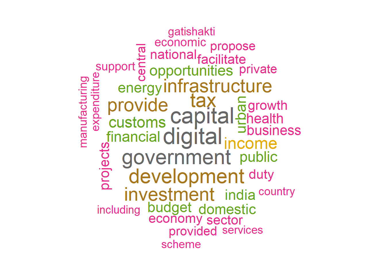

Figure 34.1: Word Cloud of FM’s Budget Speech 2022